Chapter 5 Sampling Distributions
The basic idea of the Permutation Tests is that you permute the data and compute a set of possible values of test statistic under the null hypothesis. Subsquently, you check the likelihood of the observing the realized test statistic, given these possible values. If the likelihood appears extreme, you reject the null hypothesis. The distribution of the sample statistic is called the Sampling ditribution of the statistic.
5.1 Calculating Sample Distribution
One can compute sample distributions in three ways - exact calculations, simulation and formula approximations
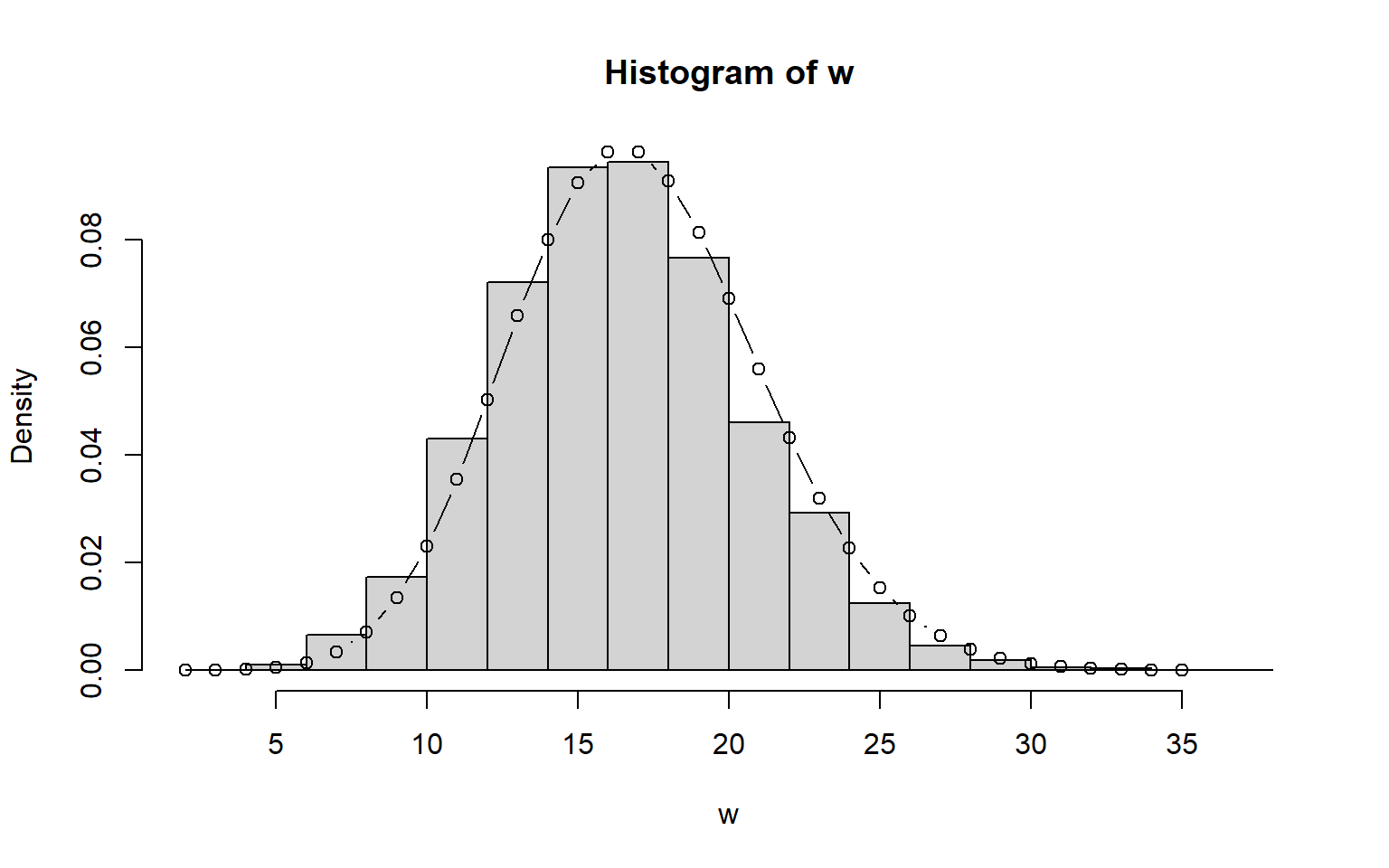
x <- rpois(10^4, 5)
y <- rpois(10^4, 12)
w <- x + y
hist(w, prob=T)
lines(2:35, dpois(2:35, 17), type="b")
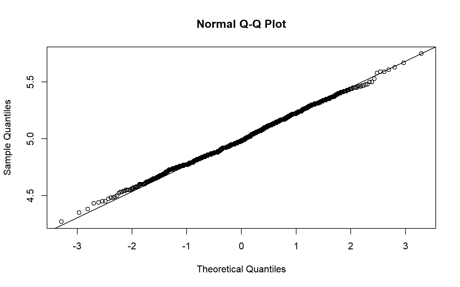
Let us simulate sample means from a poisson distribution
sample_means <- replicate(1000,{
    x <- rpois(100,5)
    mean(x)
})

qqnorm(sample_means)
qqline(sample_means)
If you look at the above plot, it is clear that the sampling distribution is normally distribution. This is not a fluke. A wide variety of statistics have approcimately normal sampling distributions if sample sizes are large enough and some other conditions are met
5.2 CLT for Binomial data
There are many instances when one encounters proportions being mentioned, and inferences being made, based on the mentioned proportions. One can invoke CLT for binomial data and then decipher whether the realized proportion is indeed a statistically significant result, as compared to the null hypothesis that we might have in mind.
Given a data, should you trust CLT or resampling ?
mean(rbinom(10^5,120,0.3)<=25)
## [1] 0.0156
CLT is an approximation. If possible, stick to resampling.
5.3 Continuity Correction
I had read about continuity correction many years ago. Was compeltely out of my working memory. When I stumbled on to the concept, after many years, I really understood it much better. It has got to do with application of CLT to small data or data whose distributions are skewed in nature. CLT is not very accurate for skewed distributions unless sample sizes are much larger, especially in the tails of distributions. Hence one needs to apply some sort of correction to the interval for which the probability needs to be computed. For example if the question asks about \(P(X>19.2)\) where \(X\) is a discrete variable, using contintuity correction, it is better to compute \(P(X>19.5)\) rather than \(P(X>=20)\)
The rule of thumb for binomial data is to use cLT, with continuity correction, if both \(np \geq 10\) and \(n(1-p) \geq 10\)
5.4 Problems with CLT
The CLT is exact if the population is normal
For non-normal populations, the biggest problem is skewness, followed by discreteness
If the population is symeetric, the sampling distribution of the mean may be close to normal for quite small \(n\)
If the population is not symmetric, then the sampling distribution may be non-normal even for a large \(n\)
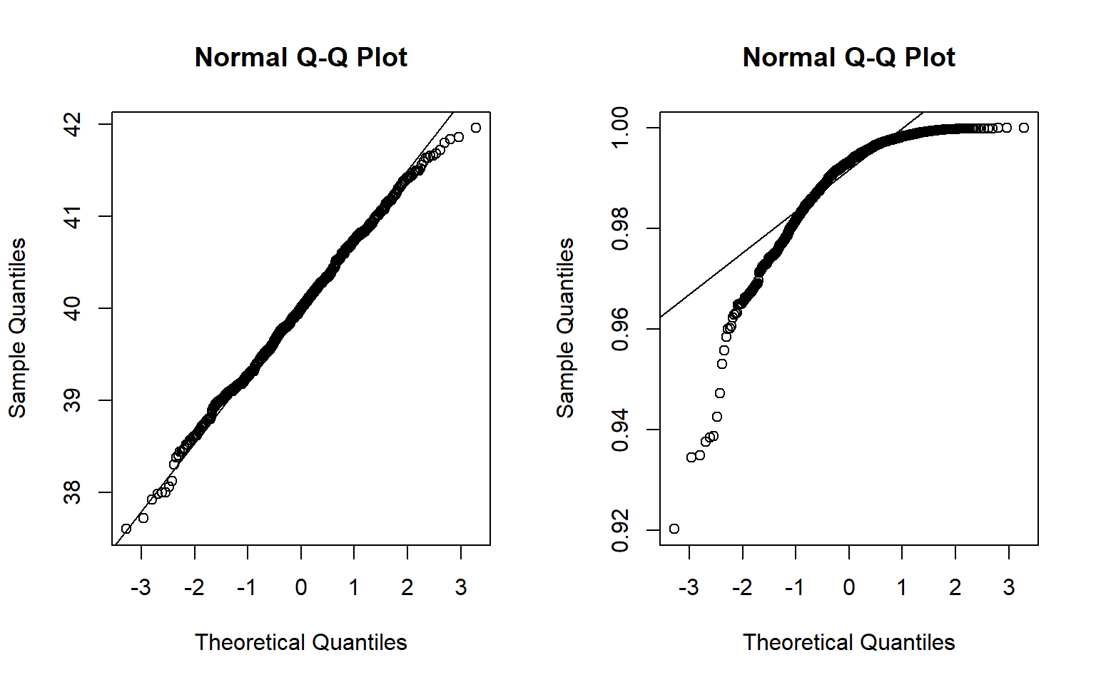
What do the above statements mean ? Let me illustrate by checking two sample statistics
- \(\overline X\) where \(X \sim Binom(100,0.5)\)
- \(\max X\) where \(X \sim Unif(0,1)\)
sample_means_1 <- replicate(1000,{
    x <- rbinom(50,100,0.4)
    mean(x)
})

sample_means_2 <- replicate(1000,{
    x <- runif(100)
    max(x)
})

par(mfrow = c(1,2))
qqnorm(sample_means_1)
qqline(sample_means_1)

qqnorm(sample_means_2)
qqline(sample_means_2)
That’s the main reason, one should not blindly apply CLT for any sample statistic
5.5 CLT for Finite populations
I had never knew that a version of CLT existed for finite populations. There is a correction factor for CLT that was provided by Jaroslav Hajek in 1960. The accuracy of the CLT version for finite populations depends on both the number of sampled and non-sampled observations.
5.6 Takeaways
- One cannot blindly invoke CLT to make probalistic inferences
- CLT crucuially depends on the assumptions on the data
- If the underlying data is skewed and discrete, one needs to apply CLT with some sort of correction. However these are all techniques that pre-date computer age. We do not have to use CLT anymore. Resample or Bootstrap away to glory.