Chapter 11 Categorical Data

df <- GSS2002[,c("Education", "DeathPenalty")]
results <- chisq.test(table(df))$statistic
chisq_resampled <- replicate(10^4, {
    idx <- sample(seq_along(df[,1]), size = dim(df)[1], T)
    temp <- table(df$Education, df$DeathPenalty[idx])
    chisq.test(temp)$statistic
})

plot(density(chisq_resampled), xlim=c(0,30))
abline(v=results)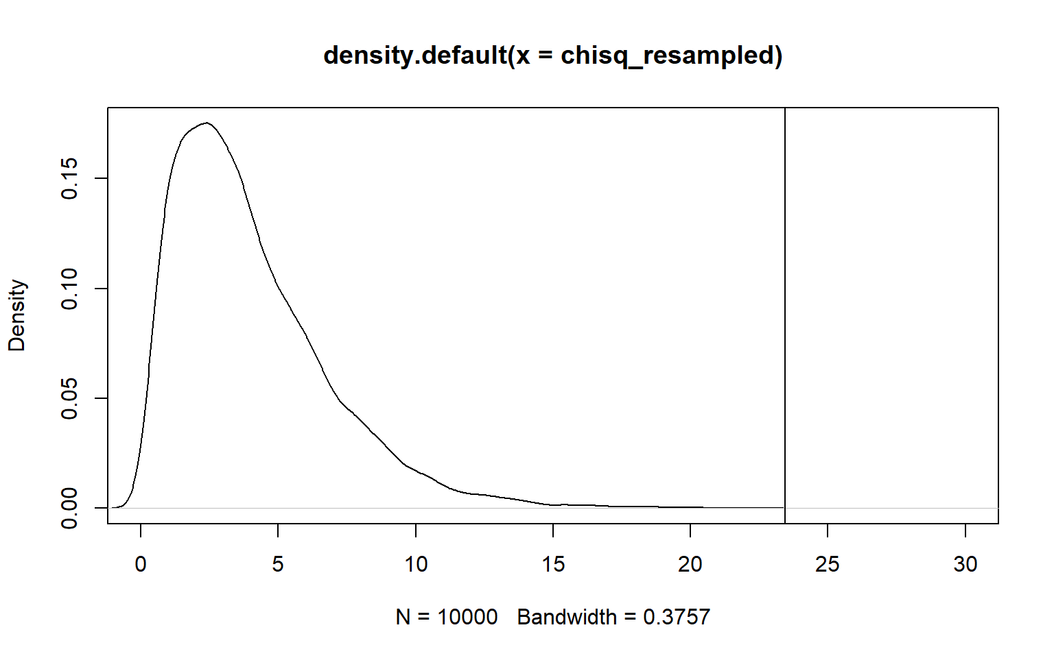

mat <- rbind(c(42, 50), c(30, 87))
chisq.test(mat)
## 
##  Pearson's Chi-squared test with Yates' continuity correction
## 
## data:  mat
## X-squared = 8.2683, df = 1, p-value = 0.004034
chisq.test(mat, correct=FALSE)
## 
##  Pearson's Chi-squared test
## 
## data:  mat
## X-squared = 9.1329, df = 1, p-value = 0.00251
fisher.test(mat)
## 
##  Fisher's Exact Test for Count Data
## 
## data:  mat
## p-value = 0.003292
## alternative hypothesis: true odds ratio is not equal to 1
## 95 percent confidence interval:
##  1.305198 4.557041
## sample estimates:
## odds ratio 
##   2.425225

11.1 Handling Contingency table data

The key question that is of interest is : whether the two variables representing the rows and columns of the table are independent. The null hypothesis in this case is that the variables are independent and hence one can work out the expected count in each cell, under the null hypothesis. Once the expected count is worked out, one can compare it to the actual counts, obtain the chisquare test statistic and compute the relevant p-value to accept or reject the null hypothesis

11.2 Permutation test

One can quickly permute the rows in one of the columns, thus obtaining a permuted sample. subsequently, one can compute a bootrstrapped distribution of the chi-squared statistic under null hypothesis and then compute the probability of seeing the observed chi-squared statistic

11.3 2 by 2 case

For a 2 by 2 contingency table, there are more than one ways to check the independence hypothesis. One of them is =Fischer exact test=

11.4 Goodness of Fit tests

The chi-squared statistic is useful in other situations where one needs to check whether the realized sample is from a specific distribution.