Chapter 10 Regression
df <- as_tibble(Spruce)
df%>%group_by(Competition, Fertilizer)%>%summarise(n())
## `summarise()` has grouped output by 'Competition'. You can override using the `.groups` argument.
## # A tibble: 4 x 3
## # Groups:   Competition [2]
##   Competition Fertilizer `n()`
##   <fct>       <fct>      <int>
## 1 C           F             18
## 2 C           NF            18
## 3 NC          F             18
## 4 NC          NF            18
df %>%mutate(diam_delta = Diameter5 - Diameter0)%>%
ggplot(aes(y=diam_delta, x = Ht.change)) + geom_point()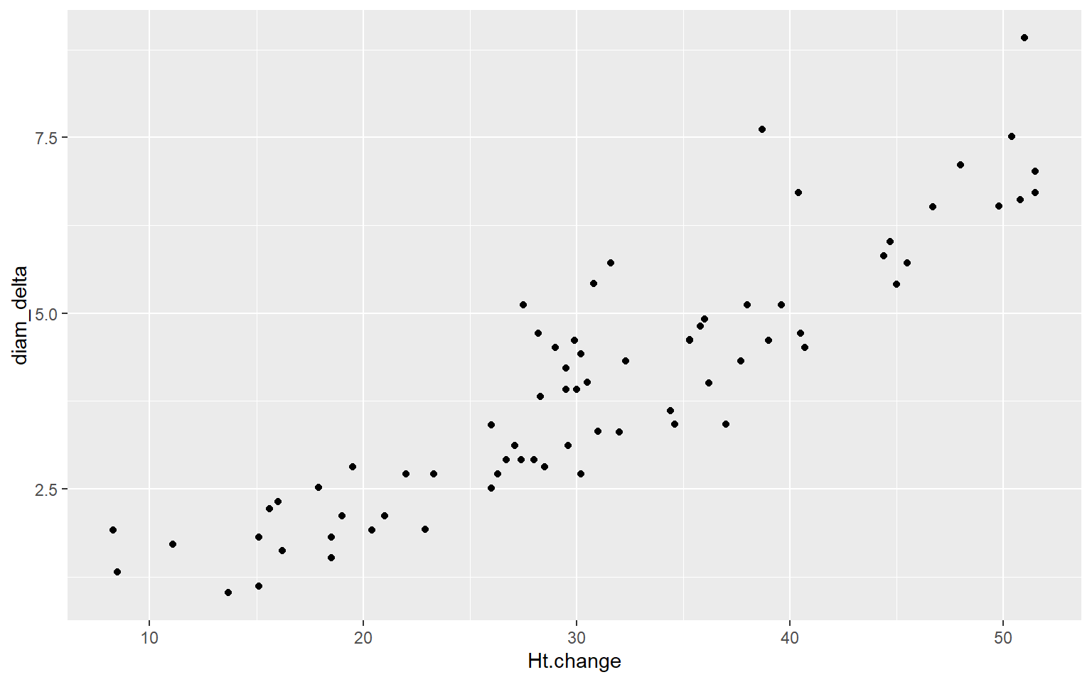
df %>%mutate(diam_delta = Diameter5 - Diameter0)%>%summarise(rho = cor(diam_delta, Ht.change))
## # A tibble: 1 x 1
##     rho
##   <dbl>
## 1 0.902
df %>%mutate(diam_delta = Diameter5 - Diameter0)%>%do(tidy(lm(diam_delta~Ht.change,.)))
## # A tibble: 2 x 5
## term estimate std.error statistic p.value
## <chr> <dbl> <dbl> <dbl> <dbl>
## 1 (Intercept) -0.519 0.274 -1.89 6.23e- 2
## 2 Ht.change 0.146 0.00835 17.5 2.98e-27Instead of looking at regular lm function, I looked up a way for a way to
perform via the tidyverse framework. Luckily I chanced upon the broom
package. This was one section that I had missed going through. Hence this is a
nice motivation for me to go through broom package.
I should go over Hadley Wichkam’s lecture on broom package where he mentions
that using broom makes it super easy to test out various models
df %>%mutate(diam_delta = Diameter5 - Diameter0)%>%
    do(tidy(lm(diam_delta~Ht.change+Fertilizer+Competition,.)))
## # A tibble: 4 x 5
##   term          estimate std.error statistic  p.value
##   <chr>            <dbl>     <dbl>     <dbl>    <dbl>
## 1 (Intercept)      1.05     0.466       2.25 2.78e- 2
## 2 Ht.change        0.104    0.0134      7.75 6.14e-11
## 3 FertilizerNF    -1.03     0.259      -3.97 1.76e- 4
## 4 CompetitionNC    0.490    0.218       2.24 2.82e- 2
model <- lm(Free~Short, Skating2010)
summary(model)
##
## Call:
## lm(formula = Free ~ Short, data = Skating2010)
##
## Residuals:
## Min 1Q Median 3Q Max
## -23.314 -6.780 0.710 6.407 21.205
##
## Coefficients:
## Estimate Std. Error t value Pr(>|t|)
## (Intercept) 7.9691 18.1175 0.440 0.664
## Short 1.7347 0.2424 7.157 3.56e-07 ***
## ---
## Signif. codes: 0 '***' 0.001 '**' 0.01 '*' 0.05 '.' 0.1 ' ' 1
##
## Residual standard error: 11.36 on 22 degrees of freedom
## Multiple R-squared: 0.6995, Adjusted R-squared: 0.6859
## F-statistic: 51.22 on 1 and 22 DF, p-value: 3.562e-07
new <- data.frame(Short = 60)
predict(model, new, interval="confidence")
## fit lwr upr
## 1 112.0494 103.4712 120.6277
predict(model, new, interval="prediction")
## fit lwr upr
## 1 112.0494 86.98175 137.117110.1 Resampling CI
pred_vals <- replicate(10^4,{
    idx <- sample(1:24,24, T)
    fitted <- lm(Free~Short, Skating2010[idx,])
    new <- data.frame(Short = 60)
    predict(fitted, new)
})
hist(pred_vals)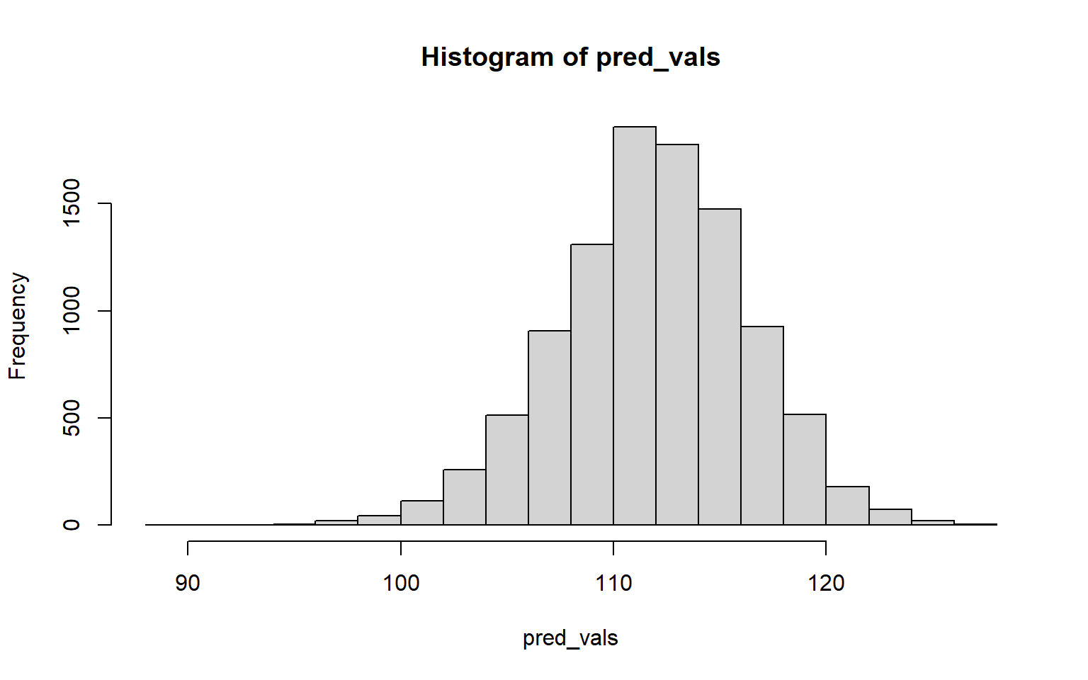
quantile(pred_vals, probs=c(0.025, 0.975))
##     2.5%    97.5%
## 102.7506 120.1658
10.2 Resampling Correlation
pred_vals <- replicate(10^4,{
    idx <- sample(1:24,24, T)
    rho_bs <- cor(Skating2010$Free, Skating2010$Short[idx])
    rho_bs
})
mean(pred_vals > cor(Skating2010$Free, Skating2010$Short))
## [1] 0
Permute one of the independent variables, compute the correlation for a large number of bootstrap samples and check whether the realized \(p-value\) is statistically significant
glm(Alcohol~ Age, data = Fatalities, family=binomial)
##
## Call:  glm(formula = Alcohol ~ Age, family = binomial, data = Fatalities)
##
## Coefficients:
## (Intercept)          Age
##    -0.12262     -0.02898
##
## Degrees of Freedom: 99 Total (i.e. Null);  98 Residual
## Null Deviance:       105.4
## Residual Deviance: 100.2     AIC: 104.2
10.3 Takeaways
- Linear Model means that the conditional distribution model is a linear model
- One must understand the difference between prediction intervals and confidence intervals
- One can use bootstrap and obtain the sampling distribution of the various coefficients in the multiple regression model
- Assumptions of the linear model
- \(x\) values are fixed
- relationship between the variables is linear
- residuals are independent
- residuals have constant variance
- residuals are normally distributed