Chapter 8 More Confidence Intervals
In the frequentist world, whenever you hear the word interval, you should automatically make a mental connection about the interval being random. 95% confidence interval means that if we repeat the same process of drawing samples and computing intervals many times, then in the long tun, 95% of the intervals will contain the true parameter
The following code shows that by repeating the process of generating random confidence intervals, one is trapping the population mean in 95% of the cases
results <- replicate(1000,{
    x <- rnorm(30,25,4)
    ci <- (mean(x) +c(-1,1)*1.96*4/sqrt(30))
    (25-ci[1])*(ci[2]-25) > 0
})
mean(results)
## [1] 0.951
x <- c(3.4, 2.9, 2.8, 5.1, 6.3, 3.9)
mean(x)+c(1,-1)*qnorm(0.05)*2.5/sqrt(length(x))
## [1] 2.387895 5.7454388.1 CI - Population SD known
If the population SD is known, one can use the sample mean and construct a confidence interval based on the fact that \({\overline X -\mu \over \sigma / \sqrt n }\) is normally distributed.
8.2 CI - Population SD unknown
results <- replicate(1000,{
    x <- rnorm(30, 25, 10)
    (mean(x)-25)/(sd(x)/sqrt(30))
}
)
qqnorm(results)
qqline(results)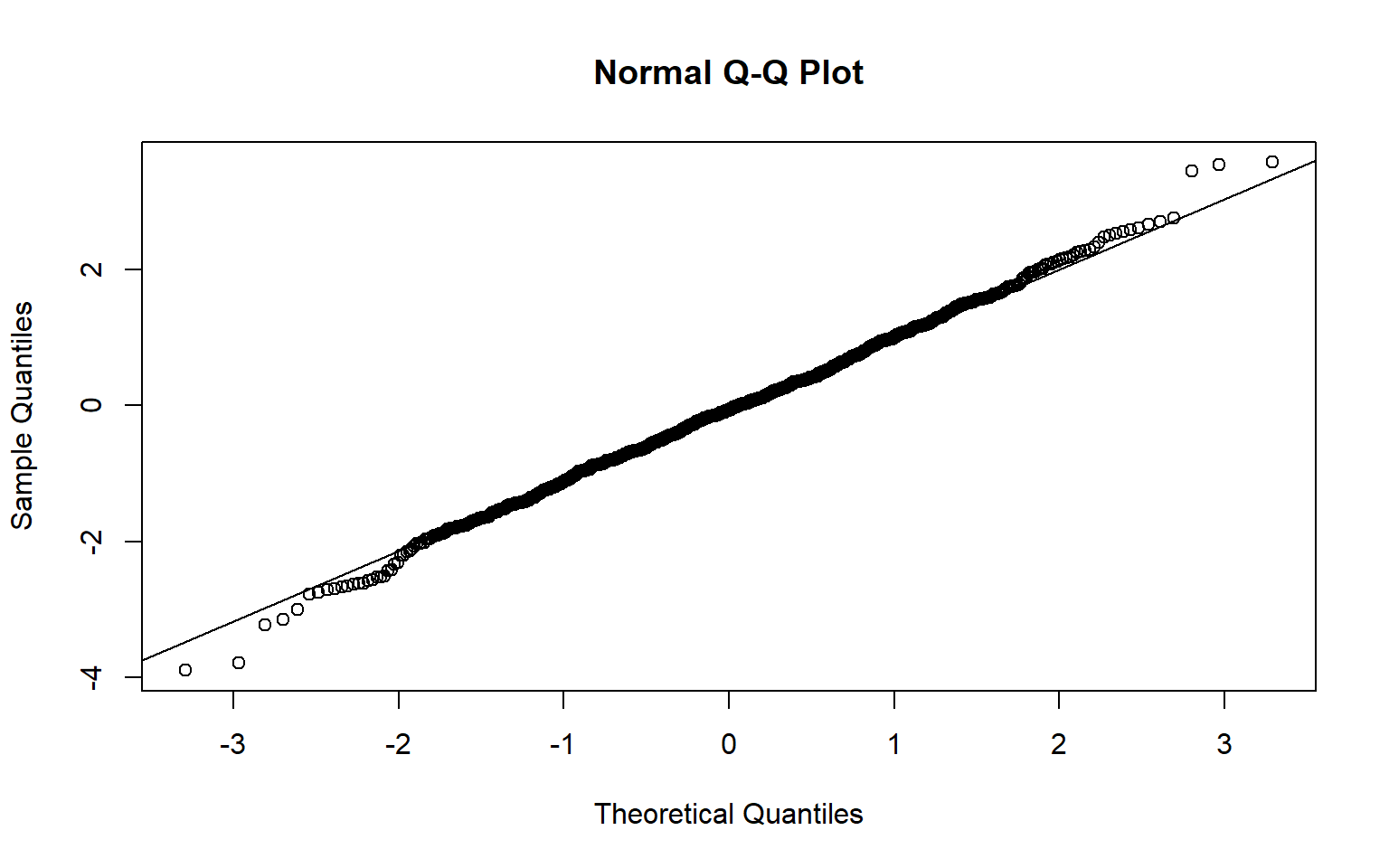
Clearly if the \(\sigma\) of the population is not known, one cannot substitute the sample standard deviation and assume the ratio of \({\overline X -\mu \over S/ \sqrt n }\) is normally distributed. It isn’t. The relevant distribution to use is Student-t distribution
results <- replicate(10000,{
    x <- rnorm(10, 25, 10)
    (mean(x)-25)/(sd(x)/sqrt(10))
}
)
Dowd::TQQPlot(results,9)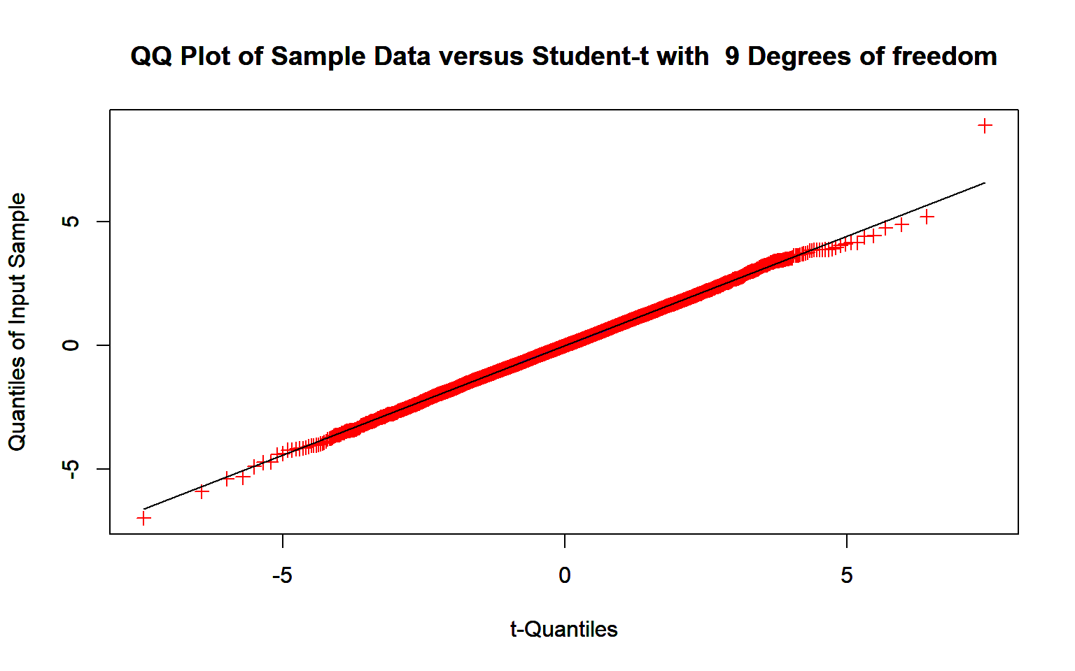
qqnorm(results, main = "check with Normal Dist")
qqline(results)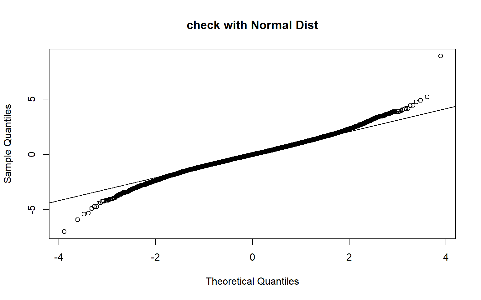
The above plots show that Normal approximation for small samples does not work.
8.3 CI for difference in means
If you have two samples and you want to figure out the CI for the difference in means, one can compute
\[ T = {(\overline X - \overline Y)-(\mu_1-\mu_2) \over \sqrt{S_1^2/n + S_2^2/n}} \]
The exact distribution of this statistic does not have a known simple distribution. It does, however, have approximately a \(t\) distribution if the populations are normal.
- I had never thought about degrees of freedom in two sample case. Indeed, what is the dof that one chooses. For two sample case, there is a Welch’s approximation that is used to choose \(\nu\) \[ \nu = {(s_1^2/n_1 + s_2^2/n_2)^2 \over (s_1^2/n_1)^2/(n_1-1) + (s_2^2/n_2)^2/(n_2-1) } \]
If we can assume that the variances of two populations are the same, then we can pool the variance
\[ S_p^2 = {(n_1-1)S_1^2 + (n_2-1)S_2^2 \over n_1 + n_2 - 2} \]
8.3.1 Pivotal Quantity
A Pivot is a random variable that depends on the sample \(X_1, X_2, \ldots X_n\) and the parameter \(\theta\), say, \(h(X_1, X_2, \ldots , \theta)\), but whose distribution does not depend on \(\theta\) or any unknown parameters
8.3.2 Location Family
Let \(F(.;\theta)\) be a family of distributions, with \(-\infty < \theta < \infty\). This is a location family if \(F(x;\theta) = H(x-\theta)\) for some function \(H\). Equivalently the distribution of \(X-\theta\) does not depend on \(\theta\). Then we call \(\theta\) ,a location parameter.
Changing the location parameters of a distribution does not change the standard deviation and shape.
8.3.3 Scale Family
Let \(F(\cdot;\theta)\) be a family of distributions, with \(0 < \theta < \infty\). This is a Scale family if \(F(x;\theta) = H(x/\theta)\) for some CDF \(H\). Equivalently the distribution of \(X/\theta\) does not depend on \(\theta\). Then we call \(\theta\) a scale parameter. For a continuous distribution \(f(x:\theta) = 1/\theta h(x\theta)\) for \(h = H^\prime\)
8.3.4 Location-Scale family
Let \(F(;\theta_L, \theta_S)\) be a family of distributions, with \(-\infty < \theta_L < \infty\) with \(0 < \theta_S < \infty\). This is a location-scale family if \(F(x;\theta_L, \theta_S) = H ( {(x-\theta_L) \over \theta_S})\). Then \(\theta_L\) and \(\theta_S\) are location and scale parameters respectively
8.4 Agresti-Coull CI
If you were shown a survey sample data and you are asked to estimate the confidence interval of some proportion relevant to the sample, then how would go about computing them ? Firstly you do not know the population variance. Hence the best unbiased estimate of \(X \sim Binom(n,p)\) is given by \(= \hat p = \hat X/n\). However the variance of this estimator is dependent of unknown \(p\), i.e. \(\sqrt{p\cdot(1-p)/n}\). Hence the confidence interval closed form is pretty messy. Agresti-Coull intervals are a convenient shortcut to computing the CI for the estimate for proportion.
The same problem plagues while inferring an CI for difference in proportions. Fortunately there is a convenient formula for this situation too.
8.5 Bootstrap CI
x <- Bangladesh$Arsenic
mu <-  mean(x)
stdev <- sd(x)
n <- length(x)
tdist <- replicate(10000, {
    y <- sample(x,n, T)
    (mean(y)-mu)/( sd(y)/sqrt(n))
}
)

mu-quantile(tdist, c(0.025, 0.975))*stdev/sqrt(n)
##      2.5%     97.5%
## 172.96173  95.38238
qqnorm(tdist)
qqline(tdist)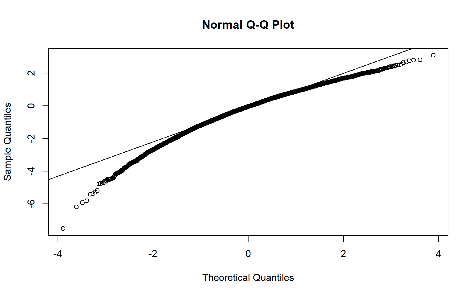
8.5.0.1 bootstrap t interval
clec <- subset(Verizon, Group=='CLEC')
ilec <- subset(Verizon, Group=="ILEC")
stats <- as_tibble(Verizon)%>%group_by(Group)%>%summarise(mu = mean(Time), sd = sd(Time), n = n())
n1 <- stats$n[1]
n2 <- stats$n[2]
tdist <- replicate(10000, {
    y1 <- sample(clec$Time,n1, T)
    y2 <- sample(ilec$Time,n2, T)
    (mean(y1)-mean(y2)-stats$mu[1] +stats$mu[2])/( sqrt(sd(y1)^2/n1+sd(y2)^2/n2 ))
}
)
mu <- (stats$mu[1] - stats$mu[2])
sig <- sqrt(stats$sd[1]^2/n1+stats$sd[2]^2/n2 )
mu-quantile(tdist, c(0.025, 0.975))*sig
##      2.5%     97.5%
## 22.134776  2.071877
8.5.0.2 Bootstrap Percentile Interval
clec <- subset(Verizon, Group=='CLEC')
ilec <- subset(Verizon, Group=="ILEC")
stats <- as_tibble(Verizon)%>%group_by(Group)%>%summarise(mu = mean(Time), sd = sd(Time), n = n())
n1 <- stats$n[1]
n2 <- stats$n[2]
tdist <- replicate(10000, {
    y1 <- sample(clec$Time,n1, T)
    y2 <- sample(ilec$Time,n2, T)
    mean(y1)-mean(y2)
}
)
quantile(tdist, c(0.025, 0.975))
##      2.5%     97.5%
##  1.773698 17.221329
8.5.0.3 formula t interval
clec <- subset(Verizon, Group=='CLEC')
ilec <- subset(Verizon, Group=="ILEC")
stats <- as_tibble(Verizon)%>%group_by(Group)%>%summarise(mu = mean(Time), sd = sd(Time), n = n())
n1 <- stats$n[1]
n2 <- stats$n[2]
welch_nu_num <- (stats$sd[1]^2/n1 + stats$sd[2]^2/n2)^2
welch_nu_den <- (stats$sd[1]^2/n1)^2/(n1-1) + (stats$sd[2]^2/n2)^2/(n2-1)
welch_nu <- welch_nu_num/welch_nu_den
print(welch_nu)
## [1] 22.34635
ci <- stats$mu[1]-stats$mu[2] +
    c(qt(0.025, welch_nu), qt(0.975, welch_nu))* sqrt(stats$sd[1]^2/n1 + stats$sd[2]^2/n2)
print(ci)
## [1] -0.3618588 16.5568985
The above stats can be replicated by using t.test
t.test(clec$Time, ilec$Time)
##
##  Welch Two Sample t-test
##
## data:  clec$Time and ilec$Time
## t = 1.9834, df = 22.346, p-value = 0.05975
## alternative hypothesis: true difference in means is not equal to 0
## 95 percent confidence interval:
##  -0.3618588 16.5568985
## sample estimates:
## mean of x mean of y
## 16.509130  8.411611
As one can see, the standard t test assumes that the population is normal and hence the derived statistic follows a \(t\) distribution with the degrees of freedom given by Welch approximation
8.6 Takeaways
- I had almost forgotten about \(t\) distribution and why it is used in hypothesis testing. If you derive any sample statistic such as mean, it is likely that the \((\overline X - \mu ) \over \sigma/\sqrt{n})\) is distributed as \(t(n-1)\) distribution
- When you know the population standard deviation, the one can use the fact that sample mean is normally distributed, and compute confidence intervals
- Margin of error for a symmetric confidence interval is the distance from the estimate to either end. The confidence itnerval is of the form estimate \(\pm\) Margin of Error
- In most real life situations, population SD, is not known. Hence one can use the fact that \((\overline X - \mu ) \over \hat \sigma/\sqrt{n})\) is distributed as \(t\) with \(n-1\) degrees of freedom
- There are 4 methods to construct CI
- Use the sample statistic and use a \(t\) distribution
- Use the sample statistic but use bootstrap standard error, and use a \(t\) distribution
- Use bootstrap percentile interval, i.e. this involves bootstrapping the statistic value, obtaining the sampling distribution of the statistic and then using the sampling distribution to read off the relevant CI’s
- Use bootstrap t test, where the sampling distribution is for the t statistic itself