Chapter 3 EDA

3.1 Basic Plots

This section starts by looking at the FlightDelays dataset

3.1.1 A basic barchart of the Carrier attribute

flights <- as_tibble(FlightDelays)
(flights%>%group_by(Carrier)%>%summarise(n()))
## # A tibble: 2 x 2
##   Carrier `n()`
## * <fct>   <int>
## 1 AA       2906
## 2 UA       1123
ggplot(flights, aes(x = Carrier))+ geom_bar() +
    scale_y_continuous(breaks = seq(0,3000,by=250))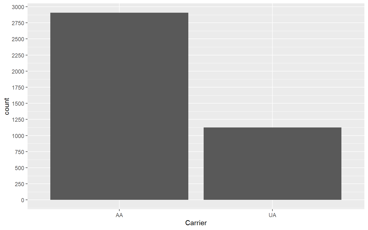

A two way contingency table between carrier and whether or not a flight was delayed more than 30 min

temp_stat <- flights%>%group_by(Carrier)%>%mutate(status = (Delayed30=='Yes'))%>%
    summarise(dl30min = mean(status), dl30min_n = sum(status), dl30min_Y = sum(!status), ct = n())
temp_stat
## # A tibble: 2 x 5
##   Carrier dl30min dl30min_n dl30min_Y    ct
## * <fct>     <dbl>     <int>     <int> <int>
## 1 AA        0.135       393      2513  2906
## 2 UA        0.182       204       919  1123

3.1.2 Flight delay in various intervals

delays <- flights %>% filter(Carrier=='UA')%>%dplyr::select(Delay)%>%unlist()
temp_stat <- as.data.frame(cut(delays,  seq(-50,450,50))%>%table())
colnames(temp_stat) <- c("time interval", "number of flights")
kbl(temp_stat) %>%
    kable_styling(bootstrap_options = "striped", full_width = F, position = "center")

time interval	number of flights
(-50,0]	722
(0,50]	249
(50,100]	86
(100,150]	39
(150,200]	14
(200,250]	7
(250,300]	3
(300,350]	2
(350,400]	1
(400,450]	0

3.1.3 Histogram of the delay times

flights %>% dplyr::filter(Carrier=='UA')%>%
    dplyr::select(Delay)%>%ggplot(aes(Delay)) +
    geom_bar()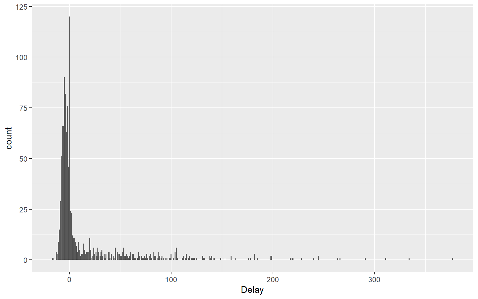

3.2 Numeric Summaries

c(mean(delays),  median(delays), sd(delays))
## [1] 15.98308 -1.00000 45.13895

summary(delays)
##    Min. 1st Qu.  Median    Mean 3rd Qu.    Max. 
##  -17.00   -5.00   -1.00   15.98   12.50  377.00

temp_stat <- flights %>% filter(Carrier=='UA')%>%dplyr::select(Delay)%>%
    summarise(n = n(), nd =n_distinct(), sd(Delay), mad(Delay), IQR(Delay), var(Delay),
              min(Delay), max(Delay), quantile(Delay, 0.3))

kbl(temp_stat) %>%
    kable_styling(bootstrap_options = "striped", full_width = F, position = "center")

n	nd	sd(Delay)	mad(Delay)	IQR(Delay)	var(Delay)	min(Delay)	max(Delay)	quantile(Delay, 0.3)
1123	0	45.13895	7.413	17.5	2037.525	-17	377	-4

3.3 Box Plots

delays <- flights %>% filter(Carrier=='UA')%>%dplyr::select(Delay,Day)
delays%>%ggplot(aes(x=Day, y=Delay))+geom_boxplot()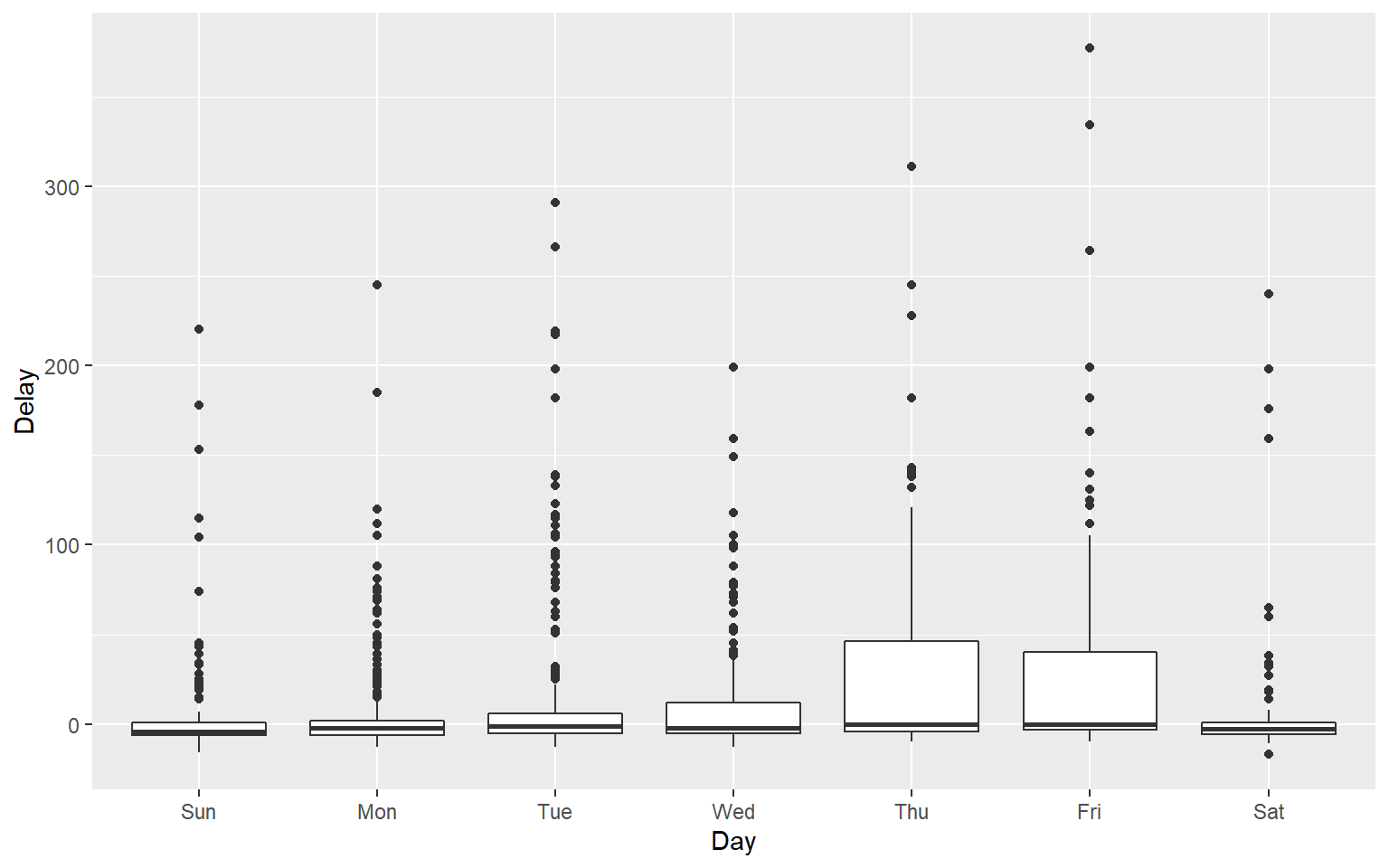

3.4 Quantile Plots

ncbirths <- as_tibble(NCBirths2004)
ncbirths%>%ggplot(aes(sample=Weight)) + geom_qq() + geom_qq_line()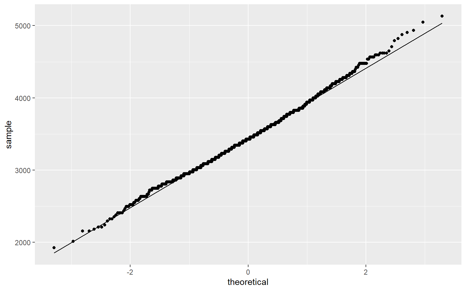

delays <- flights %>% filter(Carrier=='UA')%>%dplyr::select(Delay,Day)
delays%>%ggplot(aes(sample=Delay)) + geom_qq() + geom_qq_line()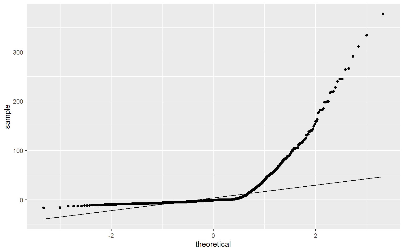

3.5 ECDF

ggplot(Beerwings, aes(Beer, color = Gender)) + stat_ecdf(geom="step")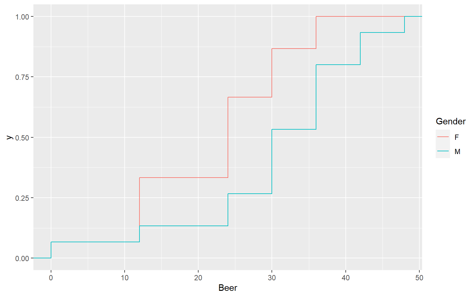

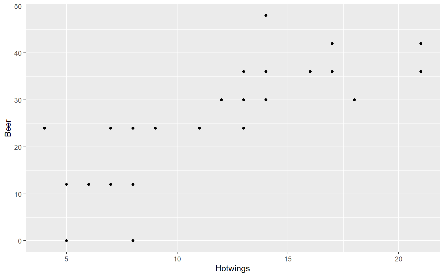
3.6 Scatterplot

ggplot(Beerwings, aes(x=Hotwings, y = Beer))+ geom_point()